ExoComp
ExoComp is a set of tools for comparing/converting/interpreting measurements of the atmospheric composition of exoplanets. Here, we run a few test and example cases.
[1]:
from exocomp import Abund
from IPython.display import display
import numpy as np
import matplotlib.pyplot as plt
Estimate [M/H] and C/O from species abundances
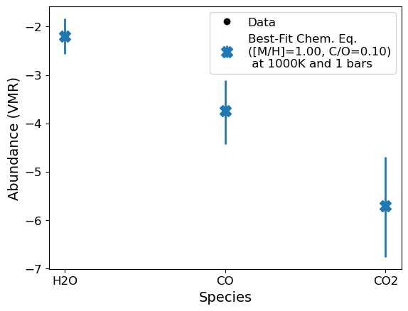
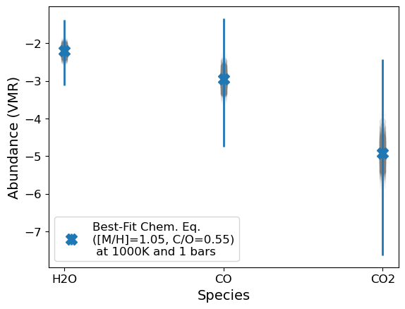
ExoComp can fit a metallicity, C/O, and refractory-to-volatile ratio to measurements of species abundances. By species abundances, I mean measurements of the abundance of individual atomic or molecular species. Below, we show that given abundances of H\(_2\)O, CO, and CO\(_2\) consistent with 10x solar metallicity and C/O = 0.5, we indeed get the expected values back.
p.s. For now, we’re also assuming we’re measuring an atmosphere at T=1000 K and at 1 bar… We’ll come back to that…
[2]:
g = Abund()
test_abunds = g.predict_abund(1.0,0.1,1000,1,adjust_C=True,verbose=True)

#Setting abundances to fit to be those at 10x solar metallicity and C/O = 0.1
g.species_abunds = test_abunds
popt,pcov,best_fit_abunds = g.convert_species_abunds(1000, 1, plot_it=True) # Need to add errors or you get weird errorbars on M/H and C/O!
H2O: -2.1935948210641625
CO: -3.740758551917497
CO2: -5.704870644717015
Consider adding errors/uncertainty to the provided measurements!
---
Best fit [M/H]: 1.000  +/- 0.376
Best fit C/O: 0.100  +/- 0.042
---
Best Fit Abundances
---
H2O: -2.1935948210641496
CO: -3.7407585519174846
CO2: -5.704870644716999
Updating bulk abundances with mean/median fit
What do we mean by metallicity and C/O?
Something that is sometimes overlooked is how exactly one defines metallicity and C/O. Metallicity is generally defined as a scaling of all elements heavier than He by some factor. But then, how does one change the C/O ratio? Some retrieval codes (PETRA, PLATON, POSEIDON) then change the C/H abundance to get the given C/O ratio, while other codes change O/H instead (pRT with pre-tabulated chemistry). The issue with this approach is that if C/O is changed after the metallicity has been set, then the new composition no longer reflects the correct metallicity! For example, in a low C/O scenario, if one sets C/H after the metallicity, then a whole bunch of carbon atoms have been removed, and the composition is now less metal enriched than it should be for the defined metallicity!
Many other codes (CHIMERA, PICASO) change the C/O in such a way that the overal metallicity remains unchanged. In a low C/O scenario, an equal number of carbon atoms are removed as oxygen atoms are added, keeping the number of atoms heavier the He the same, but lowering the C/O accordingly. Functionally:
total = O/H + C/H
C/H = C/O * total / (C/O + 1)
O/H = total / (C/O +1)
Some other codes just retrieve O/H and C/H separately and quote a metallicity based one of them or their sum (ATMO, PETRA, pRT with easyCHEM) with the latter being equivalent to the above treatment.
In ExoComp, we can adjust how we define metallicity and C/O with the adjust_C parameter. By default, ExoComp changes the C/H ratio to adjust the C/O with adjust_C = True, meaning the metallicity is equivlanet to the O/H ratio. adjust_C = False will adjust the O/H ratio to match the C/O ratio instead and adjust_C = 'Neither' will adjust the C/O while conserving the total metallicity (so metallicity is basically [(O+C)/H].
Below, the point is illustrated with the example abundances above. Our test abundances were from 10x solar metallicity and C/O = 0.1, but this was defined by adjusting C/H to obtain the given C/O (ExoComp’s default). But what if we used the other methods?
[3]:
#Default: Adjust C/H to get C/O
print('\nAdjust C/H to get C/O:')
test_abunds = g.predict_abund(1.0,0.1,1000,1,adjust_C=True,verbose=True)

#Adjust O/H to get C/O
print('\nAdjust O/H to get C/O')
test_abunds = g.predict_abund(1.0,0.1,1000,1,adjust_C=False,verbose=True)

#Adjust C/O but preserve M/H constant
print('\nAdjust C/O, but preserve M/H')
test_abunds = g.predict_abund(1.0,0.1,1000,1,adjust_C='Neither',verbose=True)
Adjust C/H to get C/O:
H2O: -2.1935948210641625
CO: -3.740758551917497
CO2: -5.704870644717015

Adjust O/H to get C/O
H2O: -1.3902937541418852
CO: -2.5332379909695253
CO2: -3.674217006349617

Adjust C/O, but preserve M/H
H2O: -2.015773925761302
CO: -3.4567423478404438
CO2: -5.241189750109873
They’re so different! The different methods can result in almost 2 orders of magntiude difference in expected abundances for CO\(_2\). What would the corresponding fits to metallicity and C/O be?
[4]:
print('\nAdjust O/H to get C/O')
popt,pcov,best_fit = g.convert_species_abunds(1000, 1, plot_it=False, adjust_C=False)

print('\nAdjust C/O, but preserve M/H')
popt,pcov,best_fit = g.convert_species_abunds(1000, 1, plot_it=False, adjust_C='Neither')
Adjust O/H to get C/O
Consider adding errors/uncertainty to the provided measurements!
---
Best fit [M/H]: 0.261  +/- 2.590
Best fit C/O: 0.121  +/- 0.074
---
Best Fit Abundances
---
H2O: -2.1933361378098493
CO: -3.7405011251604616
CO2: -5.705127695480436
Updating bulk abundances with mean/median fit

Adjust C/O, but preserve M/H
Consider adding errors/uncertainty to the provided measurements!
---
Best fit [M/H]: 0.822  +/- 0.116
Best fit C/O: 0.108  +/- 0.052
---
Best Fit Abundances
---
H2O: -2.1934883965417504
CO: -3.7406528166603428
CO2: -5.704976246285373
Updating bulk abundances with mean/median fit
We can obtain the same species abundances, but the metallicity or C/O we infer is wildly different from the 10x solar and 0.1 C/O we input using the other C/O definition!
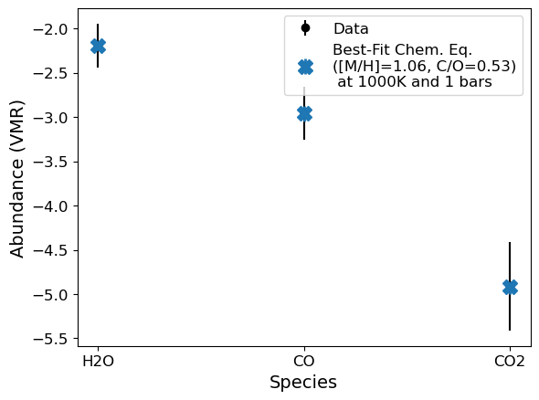
Adding uncertainties into our measurements
Any good measurement will have an associated uncertainty. We can incorporate these into our fits. exocomp handles symmetric errors, asymmetric errors, and the ability to input posterior samples. The latter can take a bit of computation if there are lots of samples because it is using curve_fit to fit each sample. You can reduce the number of fitted samples by defining posterior_samples. Let’s take a look:
[5]:
# Symmetric errors
g = Abund(species_abunds={'H2O': -2.196454926078874, 'CO': -2.95559683423187, 'CO2': -4.9118293333092335},
          species_errs={'H2O': 0.25, 'CO': 0.3, 'CO2': 0.5})
popt,pcov,best_fit_abunds = g.convert_species_abunds(1000, 1, plot_it=True)
---
Best fit [M/H]: 1.056  +/- 0.001
Best fit C/O: 0.531  +/- 0.116
---
Best Fit Abundances
---
H2O: -2.19516931830578
CO: -2.9537410033888496
CO2: -4.916949667855418
Chi^2 = 0.00016958376897597855, Reduced Chi^2 = 8.479188448798927e-05
Updating bulk abundances with mean/median fit
[6]:
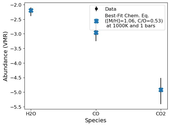
# Asymmetric errors - will use scipy.optimize.fmin rather than curve_fit
g = Abund(species_abunds={'H2O': -2.196454926078874, 'CO': -2.95559683423187, 'CO2': -4.9118293333092335},
          species_errs={'H2O': [0.2,0.1], 'CO': [0.3,0.3], 'CO2': [0.5,0.4]})
popt,pcov,best_fit_abunds = g.convert_species_abunds(1000, 1, plot_it=True)
Optimization terminated successfully.
         Current function value: 0.000195
         Iterations: 42
         Function evaluations: 82
---
Best fit [M/H]: 1.055
Best fit C/O: 0.534
Chi^2 = 39896627.976812825, Reduced Chi^2 = 19948313.988406412
---
Best Fit Abundances
---
H2O: -2.196227532130406
CO: -2.953466315741787
CO2: -4.917735870799223
Updating bulk abundances with mean/median fit
[7]:
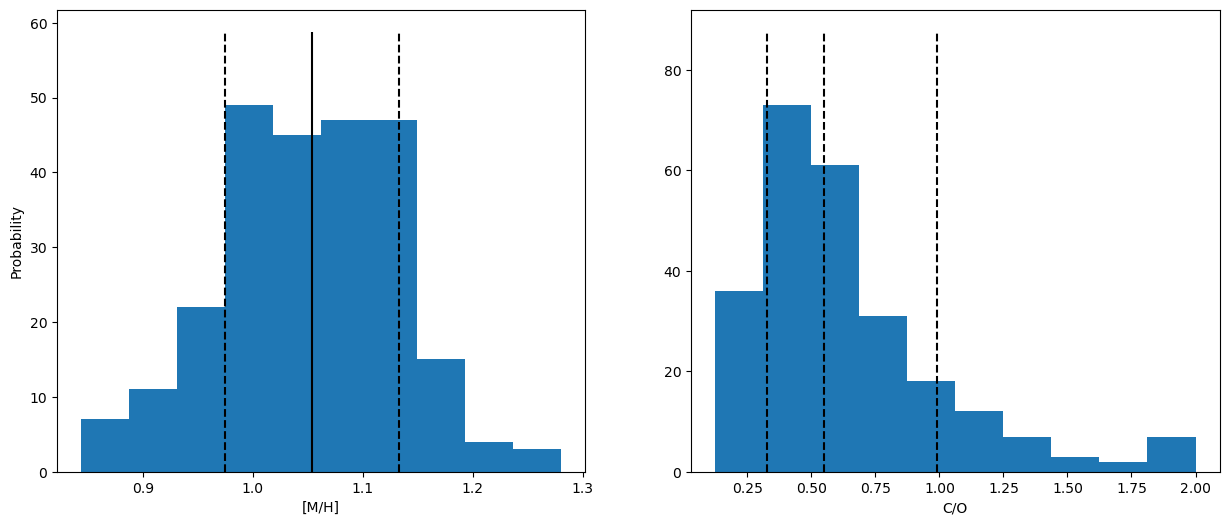
# Posterior samples
h2o_err = np.random.normal(-2.2,0.1,1000)
co_err = np.random.normal(-2.96,0.2,1000)
co2_err = np.random.normal(-4.91,0.3,1000)

g = Abund(species_abunds={'H2O': -2.196454926078874, 'CO': -2.95559683423187, 'CO2': -4.9118293333092335},
          species_errs={'H2O': h2o_err, 'CO': co_err, 'CO2': co2_err})
popt,pcov,best_fit_abunds = g.convert_species_abunds(1000, 1, plot_it=True, posterior_samples=250) # Doesn't matter if C/O adjusts C or O here
Running on 250 samples... May take a moment if >10
---
Metallicity - Median: 1.0539, Lower bound: 0.9747, Upper bound: 1.1328
C/O - Median: 0.5501, Lower bound: 0.3275, Upper bound: 0.9885
---
Median Fit Abundances
---
H2O: -2.1996638510444004
CO: -2.9443853957585833
CO2: -4.912042947072754
Updating bulk abundances with mean/median fit
Adding refractories
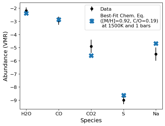
Many folks [1,2,3,4] have pointed out the utility of measuring refractory elements to understand processes like 1) cloud formation, 2) rainout, and 3) planet formation. With exocomp, we can add measurements of any refractory element (basically anything past oxygen on the periodic table) to constrain the refractory-to-volatile ratio by setting fit_refvol=True. We can also just use the additional measurements to further constrain the metallicity. Both cases are shown below.
[8]:
# Using Sulfur and Sodium to further constrain the metallicity
# Symmetric errors
g = Abund(species_abunds={'H2O': -2.20, 'CO': -2.96, 'CO2': -4.91,'S':-9.0,'Na':-5.5},
          species_errs={'H2O': 0.25, 'CO': 0.3, 'CO2': 0.5, 'S':0.3, 'Na':0.5})
popt,pcov,best_fit_abunds = g.convert_species_abunds(1500, 1, plot_it=True) # We need to increase the temperature so S is not condensed...
---
Best fit [M/H]: 0.921  +/- 0.000
Best fit C/O: 0.192  +/- 0.000
---
Best Fit Abundances
---
H2O: -2.3801603061726535
CO: -2.875074266378856
CO2: -5.596428406271661
S: -8.628516809069882
Na: -4.680052969697716
Chi^2 = 6.706780369973133, Reduced Chi^2 = 1.6766950924932833
Updating bulk abundances with mean/median fit
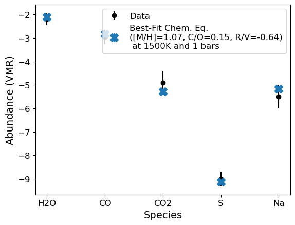
[9]:
# Using Sulfur to further co
# Symmetric errors
g = Abund(species_abunds={'H2O': -2.20, 'CO': -2.96, 'CO2': -4.91,'S':-9.0,'Na':-5.5},
          species_errs={'H2O': 0.25, 'CO': 0.3, 'CO2': 0.5, 'S':0.3, 'Na':0.5})
popt,pcov,best_fit_abunds = g.convert_species_abunds(1500, 1, plot_it=True, fit_refvol=True) # Doesn't matter if C/O adjusts C or O here
---
Best fit [M/H]: 1.069  +/- 0.001
Best fit C/O: 0.152  +/- 0.000
Best fit R/V: -0.639  +/- 0.009
---
Best Fit Abundances
---
H2O: -2.107080366027173
CO: -2.8282389963421037
CO2: -5.274885927979525
S: -9.118131964522485
Na: -5.171683908984855
Chi^2 = 1.449834641902057, Reduced Chi^2 = 0.3624586604755142
Updating bulk abundances with mean/median fit
Changing our solar reference abundances
Metallicity, as defined here, is always relative to a reference abundance. Usually this is “solar composition” of some variety, but sometimes we have enough information about the host star to use the stellar abundances as our reference. Unfortunately, if we want to compare retrieval results, the reference abundances used in various studies or retrieval codes varies considerably!
When it comes to solar abundances, many references exist. ExoComp has abundances from Lodders et al. 2010, 2021, and 2025, Asplund et al. 2005, 2009, 2021, and Caffau et al. 2011. These are listed in exocomp.Abund.possible_solars. In exocomp.Abund.define_stellar, one can input any known stellar elemental abundances to be used in the calculations (whatever is defined in exocomp.Abund.stellar will be used for anything not defined).
Let’s look at our example at 10x solar metallicity and \(\mathrm{C/O} = 0.1\), but with different solar abundances. The default we’ve been using so far is the most recent reference, Lodders et al. 2025. Again, the default treatment of C/O is to vary C/H.
[10]:
# Our original example used Lodders+ 2025 to get abundances of H2O, CO, and CO2 at 10x solar metallicity and C/O=0.1
# Again at 1000 K and 1 bar
print('Lodders+ 2025')
g = Abund(species_abunds={'H2O': -2.196454926078874, 'CO': -2.95559683423187, 'CO2': -4.9118293333092335},
          species_errs={'H2O': 0.1, 'CO': 0.1, 'CO2': 0.1}, solar='Lodders25')
popt,pcov,best_fit_abunds = g.convert_species_abunds(1000, 1, plot_it=False)

print('\nAsplund+ 2009')
g = Abund(species_abunds={'H2O': -2.196454926078874, 'CO': -2.95559683423187, 'CO2': -4.9118293333092335},
          species_errs={'H2O': 0.1, 'CO': 0.1, 'CO2': 0.1}, solar='Asplund09')
popt,pcov,best_fit_abunds = g.convert_species_abunds(1000, 1, plot_it=False)

print('\nLodders+ 2010')
g = Abund(species_abunds={'H2O': -2.196454926078874, 'CO': -2.95559683423187, 'CO2': -4.9118293333092335},
          species_errs={'H2O': 0.1, 'CO': 0.1, 'CO2': 0.1}, solar='Lodders10')
popt,pcov,best_fit_abunds = g.convert_species_abunds(1000, 1, plot_it=False)
Lodders+ 2025
---
Best fit [M/H]: 1.001  +/- 0.000
Best fit C/O: 0.500  +/- 0.002
---
Best Fit Abundances
---
H2O: -2.196456010547247
CO: -2.9555979209728966
CO2: -4.911828253745222
Chi^2 = 3.522536165426771e-10, Reduced Chi^2 = 1.7612680827133854e-10
Updating bulk abundances with mean/median fit

Asplund+ 2009
---
Best fit [M/H]: 1.058  +/- 0.000
Best fit C/O: 0.529  +/- 0.002
---
Best Fit Abundances
---
H2O: -2.193703402171143
CO: -2.9528386553972754
CO2: -4.914568928043371
Chi^2 = 0.0022683813605737756, Reduced Chi^2 = 0.0011341906802868878
Updating bulk abundances with mean/median fit

Lodders+ 2010
---
Best fit [M/H]: 1.095  +/- 0.000
Best fit C/O: 0.521  +/- 0.002
---
Best Fit Abundances
---
H2O: -2.193696515820324
CO: -2.9528316475014313
CO2: -4.914575904597135
Chi^2 = 0.0022798738648195493, Reduced Chi^2 = 0.0011399369324097746
Updating bulk abundances with mean/median fit
Case Study: WASP-77A b
Let’s look at a real-world example of this. Line et al. 2022 measured relatively high precision oxygen and carbon abundances in WASP-77Ab. Below, we use exocomp.Abund.define_solar() to re-define the reference oxygen and carbon abundances with values measured from Regginai et al. 2022.
[19]:
from exocomp import Abund
from IPython.display import display
import numpy as np
import matplotlib.pyplot as plt

# initialize Abund instance with retrieval defined so we get correct mh_type and co_type
g = Abund(retrieval='CHIMERA',solar = 'Asplund09')
#display(g.solar_abundances_orig)

# convert bulk abundances to elemental abundances
g.convert_bulk_abundance(-0.48,0.59,mh_err=[0.12,0.14],co_err=[0.08,0.08],solar = 'Asplund09')
#g.convert_bulk_abundance(-0.41,0.46,mh_err=[0.14,0.14],co_err=[0.08,0.08],solar = 'Asplund09') #Accounting for rainout

print('Asplund+ 2009 Solar Abundances')
print(f'[O/H] = {g.bulk_abunds['O']-g.solar_abundances['O'][0]} +/- {np.max(g.bulk_errs['O'])}') #errors here assume O/H and C/H are uncorrelated...
print(f'[C/H] = {g.bulk_abunds['C']-g.solar_abundances['C'][0]} +/- {np.max(g.bulk_errs['C'])}')
print(f'C/O_p = {10**g.bulk_abunds['C']/10**g.bulk_abunds['O']} +/- 0.08') #C/O errors not saved elsewhere
print(f'C/O_* = {(10**g.solar_abundances['C'][0]/10**g.solar_abundances['O'][0])}')
print(f'(C/O_p)/(C/O_*) = {(10**g.bulk_abunds['C']/10**g.bulk_abunds['O'])/(10**g.solar_abundances['C'][0]/10**g.solar_abundances['O'][0])}')

# redefine solar based on Reggiani et al. 2022
g.define_stellar({'O':(8.92,0.23),'C':(8.56,0.1)})

print('\nReggiani+ Stellar Abundances')
print(f'[O/H] = {g.bulk_abunds['O']-g.solar_abundances['O'][0]} +/- {np.max(g.bulk_errs['O'])}')
print(f'[C/H] = {g.bulk_abunds['C']-g.solar_abundances['C'][0]} +/- {np.max(g.bulk_errs['C'])}')
print(f'[(C+O)/H] = {np.log10((10**g.bulk_abunds['C']+10**g.bulk_abunds['O'])/((10**g.solar_abundances['C'][0]+10**g.solar_abundances['O'][0])))} +/- \
    {np.sqrt(np.max(g.bulk_errs['C'])**2+np.max(g.bulk_errs['O'])**2)}')

print(f'C/O_p = {10**g.bulk_abunds['C']/10**g.bulk_abunds['O']} +/- 0.08') #C/O errors not saved elsewhere
print(f'C/O_* = {(10**g.solar_abundances['C'][0]/10**g.solar_abundances['O'][0])}')
print(f'(C/O_p)/(C/O_*) = {(10**g.bulk_abunds['C']/10**g.bulk_abunds['O'])/(10**g.solar_abundances['C'][0]/10**g.solar_abundances['O'][0])}')
Using Asplund09 solar abundances
Asplund+ 2009 Solar Abundances
[O/H] = -0.4911940877550265 +/- 0.14
[C/H] = -0.460342076112882 +/- 0.14
C/O_p = 0.5900000000000007 +/- 0.08
C/O_* = 0.5495408738576247
(C/O_p)/(C/O_*) = 1.0736235065798911

Reggiani+ Stellar Abundances
[O/H] = -0.7211940877550269 +/- 0.14
[C/H] = -0.5903420761128828 +/- 0.14
[(C+O)/H] = -0.6771073802690852 +/-     0.19798989873223333
C/O_p = 0.5900000000000007 +/- 0.08
C/O_* = 0.43651583224016655
(C/O_p)/(C/O_*) = 1.351611915132986
This is a super interesting case, where if we compared WASP-77Ab’s C/O measurement to solar abundances, we would conclude that it has a C/O consistent with solar. But if we compare the C/O in the planet to new, state-of-the-art measurements of the C/O ratio of the star, then we see that the planet is actually more highly enriched in carbon than the star!
We can calculate the elemental ratios relative to solar or stellar with the exocomp.Abund.solar_ratio_calc() routine, which outputs the elemental abundances relative to our reference abundances. However, we do not include the errors here because the uncertainty in the C/H and O/H abundances of WASP-77A are well-correlated such that their individual absolute abundances as input here are not measured as precise as their ratio.
In any case:
[12]:
g = Abund(retrieval='CHIMERA',solar = 'Asplund09')
#display(g.solar_abundances_orig)

# convert bulk abundances to elemental abundances
g.convert_bulk_abundance(-0.48,0.59,mh_err=[0.12,0.14],co_err=[0.08,0.08],solar = 'Asplund09')

solar_ratios, solar_ratios_err = g.solar_ratio_calc()
ratio = 10**solar_ratios['C']/10**solar_ratios['O']
#exponent_error = np.sqrt(solar_ratios_err['C']**2 + solar_ratios_err['O']**2)
#ratio_error = ratio * np.log(10) * exponent_error
print(f'C/O relative to solar: {ratio}') #Note that

#Redefine O and C using Reganni et al. stellar abundances
g.define_stellar({'O':(8.92,0.23),'C':(8.56,0.1)})
solar_ratios, solar_ratios_err = g.solar_ratio_calc()
ratio = 10**solar_ratios['C']/10**solar_ratios['O']
#exponent_error = np.sqrt(solar_ratios_err['C']**2 + solar_ratios_err['O']**2)
#ratio_error = ratio * np.log(10) * exponent_error
print(f'C/O relative to stellar: {ratio}') #Note that
Using Asplund09 solar abundances
C/O relative to solar: 1.073623506579891
C/O relative to stellar: 1.351611915132986
Let’s do this again with the values from August et al. 2023 using JWST/NIRSpec data on the same system.
[20]:
# initialize Abund instance with retrieval defined so we get correct mh_type and co_type
g = Abund(retrieval='PLATON')
#display(g.solar_abundances_orig)

# convert bulk abundances to elemental abundances
g.convert_bulk_abundance(-0.91,0.36,mh_err=[0.16,0.24],co_err=[0.09,0.10])
#g.convert_bulk_abundance(-0.41,0.46,mh_err=[0.14,0.14],co_err=[0.08,0.08],solar = 'Asplund09') #Accounting for rainout

print('Asplund+ 2009 Solar Abundances')
print(f'[O/H] = {g.bulk_abunds['O']-g.solar_abundances['O'][0]} +/- {np.max(g.bulk_errs['O'])}') #errors here assume O/H and C/H are uncorrelated...
print(f'[C/H] = {g.bulk_abunds['C']-g.solar_abundances['C'][0]} +/- {np.max(g.bulk_errs['C'])}')
print(f'C/O_p = {10**g.bulk_abunds['C']/10**g.bulk_abunds['O']} +/- 0.08') #C/O errors not saved elsewhere
print(f'C/O_* = {(10**g.solar_abundances['C'][0]/10**g.solar_abundances['O'][0])}')
print(f'(C/O_p)/(C/O_*) = {(10**g.bulk_abunds['C']/10**g.bulk_abunds['O'])/(10**g.solar_abundances['C'][0]/10**g.solar_abundances['O'][0])}')

# redefine solar based on Reggiani et al. 2022
g.define_stellar({'O':(8.92,0.23),'C':(8.56,0.1)})

print('\nReggiani+ Stellar Abundances')
print(f'[O/H] = {g.bulk_abunds['O']-g.solar_abundances['O'][0]} +/- {np.max(g.bulk_errs['O'])}')
print(f'[C/H] = {g.bulk_abunds['C']-g.solar_abundances['C'][0]} +/- {np.max(g.bulk_errs['C'])}')
print(f'[(C+O)/H] = {np.log10((10**g.bulk_abunds['C']+10**g.bulk_abunds['O'])/((10**g.solar_abundances['C'][0]+10**g.solar_abundances['O'][0])))} +/- \
    {np.sqrt(np.max(g.bulk_errs['C'])**2+np.max(g.bulk_errs['O'])**2)}')
print(f'C/O_p = {10**g.bulk_abunds['C']/10**g.bulk_abunds['O']} +/- 0.08') #C/O errors not saved elsewhere
print(f'C/O_* = {(10**g.solar_abundances['C'][0]/10**g.solar_abundances['O'][0])}')
print(f'(C/O_p)/(C/O_*) = {(10**g.bulk_abunds['C']/10**g.bulk_abunds['O'])/(10**g.solar_abundances['C'][0]/10**g.solar_abundances['O'][0])}')
Using Asplund09 solar abundances
Asplund+ 2009 Solar Abundances
[O/H] = -0.9100000000000001 +/- 0.24
[C/H] = -1.0936974992327126 +/- 0.26
C/O_p = 0.3600000000000003 +/- 0.08
C/O_* = 0.5495408738576247
(C/O_p)/(C/O_*) = 0.6550923090995944

Reggiani+ Stellar Abundances
[O/H] = -1.1400000000000006 +/- 0.24
[C/H] = -1.2236974992327134 +/- 0.26
[(C+O)/H] = -1.1637715084642928 +/-     0.3538361202590827
C/O_p = 0.3600000000000003 +/- 0.08
C/O_* = 0.43651583224016655
(C/O_p)/(C/O_*) = 0.824712354996398
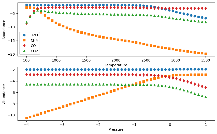
Sensitivity to Temperature and Pressure
A given metallicity and C/O ratio will correspond to a different set of species abundances depending on the temperature and pressure of an atmosphere. The two biggest reasons are the CH\(_4\)-to-CO transition from low-to-high temperatures and thermal dissociation of molecules at high temperatures. You can see both these at work in the plots below, showing how abundances change at 10 times solar metallicity 1) at 1 mbar as a function of temperture and 2) at 1000 K as a function of pressure.
There will be a sweet-spot where we can be a bit more confident in our inferences because the chemistry isn’t quite so sensitive to the assumed pressure and temperature. For example, above 1000 K, we can be confident that we’re safely in the CO-dominated regime and below 2500 K, we can be confident that we’re not subject to much thermal dissociation. As with this whole exercise, disequilbrium chemistry processes like vertical mixing and photochemistry can also influence our inferences, so be aware of that too.
[13]:
temps = np.linspace(500,3500)
pressures = np.linspace(-4,1)
cs = ['#1f77b4', '#ff7f0e', '#d62728','#2ca02c', '#9467bd', '#8c564b', '#e377c2', '#7f7f7f', '#bcbd22', '#17becf'] #colors

fig,ax = plt.subplots(2,1,figsize=(10,6))
for i,t in enumerate(temps):
    test_abunds = g.predict_abund(1.0,0.1,t,1e-3,adjust_C=True,verbose=False,species=['H2O','CO','CO2','CH4'])
    ax[0].plot(t,test_abunds['H2O'],'o',color=cs[0],label = 'H2O' if i == 0 else '')
    ax[0].plot(t,test_abunds['CH4'],'s',color=cs[1],label = 'CH4' if t == np.min(temps) else '')
    ax[0].plot(t,test_abunds['CO'],'d',color=cs[2],label = 'CO' if t == np.min(temps) else '')
    ax[0].plot(t,test_abunds['CO2'],'^',color=cs[3],label = 'CO2' if t == np.min(temps) else '')

ax[0].set_xlabel('Temperature')
ax[0].set_ylabel('Abundance')
ax[0].legend()

for p in pressures:
    test_abunds = g.predict_abund(1.0,0.1,1000,10**p,adjust_C=True,verbose=False,species=['H2O','CO','CO2','CH4'])
    ax[1].plot(p,test_abunds['H2O'],'o',color=cs[0],label = 'H2O' if t == np.min(temps) else '')
    ax[1].plot(p,test_abunds['CH4'],'s',color=cs[1],label = 'CH4' if t == np.min(temps) else '')
    ax[1].plot(p,test_abunds['CO'],'d',color=cs[2],label = 'CO' if t == np.min(temps) else '')
    ax[1].plot(p,test_abunds['CO2'],'^',color=cs[3],label = 'CO2' if t == np.min(temps) else '')

ax[1].set_xlabel('Pressure')
ax[1].set_ylabel('Abundance')
[13]:
Text(0, 0.5, 'Abundance')
Thus, on the flip-side, our inference of the metallicity and C/O will change for a given set of species abundances, depending on the pressure and temperature that we assume those abundances are representative of. Below, you can see that assuming a (very) wrong temperature will give us the wrong metallicity and C/O and abundances that don’t fit very well!
Assuming the wrong pressure is a little more forgiving, but our C/O estimate is off by a factor of four because there’s actually more CH\(_4\) and less CO and CO\(_2\) at depth. Remember what we said above though, and if you chose to define C/O differently, you’ll be biased in a different way! The only reason our metallicity didn’t change when assuming a different pressure was because H\(_2\)O is relatively robust to pressure in this temperature regime and the metallicity was essentially defined as [O/H]. If we define things differently, our estimates are even more messed up.
[14]:
# Assume our fiducial 10x solar metallicity, C/O = 0.1, T=1000K and pressure = 1bar
test_abunds = g.predict_abund(1.0,0.1,1000,1,adjust_C=True,verbose=False)

g = Abund(species_abunds=test_abunds,
          species_errs={'H2O': 0.1, 'CO': 0.1, 'CO2': 0.1}, solar='Lodders25')

print('Fitting for bulk abundances at the correct T=1000K and P=1bar')
popt,pcov,best_fit_abunds = g.convert_species_abunds(1000, 1, plot_it=False)

print('\nFitting for bulk abundances at the wrong T=3000K')
popt,pcov,best_fit_abunds = g.convert_species_abunds(3000, 1, plot_it=False)

print('\nFitting for bulk abundances at the wrong P=1e-4 bar')
popt,pcov,best_fit_abunds = g.convert_species_abunds(1000, 1e-4, plot_it=False)

print('\nFitting for bulk abundances at the wrong P=1e-4 bar, defining C/O by O/H')
popt,pcov,best_fit_abunds = g.convert_species_abunds(1000, 1e-4, plot_it=False, adjust_C=False)

print('\nFitting for bulk abundances at the wrong P=1e-4 bar, defining C/O consistently with M/H')
popt,pcov,best_fit_abunds = g.convert_species_abunds(1000, 1e-4, plot_it=False, adjust_C='Neither')
Fitting for bulk abundances at the correct T=1000K and P=1bar
---
Best fit [M/H]: 1.219  +/- 0.000
Best fit C/O: 0.085  +/- 0.000
---
Best Fit Abundances
---
H2O: -1.9269685283939144
CO: -3.3145903720687953
CO2: -4.999774192669719
Chi^2 = 0.002798471471121238, Reduced Chi^2 = 0.001399235735560619
Updating bulk abundances with mean/median fit

Fitting for bulk abundances at the wrong T=3000K
---
Best fit [M/H]: 1.531  +/- 0.000
Best fit C/O: 0.033  +/- 0.000
---
Best Fit Abundances
---
H2O: -1.6024375664538895
CO: -3.004024008397868
CO2: -5.309866587763058
Chi^2 = 29.21826991328298, Reduced Chi^2 = 14.60913495664149
Updating bulk abundances with mean/median fit

Fitting for bulk abundances at the wrong P=1e-4 bar
---
Best fit [M/H]: 1.219  +/- 0.000
Best fit C/O: 0.031  +/- 0.000
---
Best Fit Abundances
---
H2O: -1.926799365189687
CO: -3.314416514885071
CO2: -4.999944236575657
Chi^2 = 0.0024938703370249184, Reduced Chi^2 = 0.0012469351685124592
Updating bulk abundances with mean/median fit

Fitting for bulk abundances at the wrong P=1e-4 bar, defining C/O by O/H
---
Best fit [M/H]: 0.011  +/- 0.000
Best fit C/O: 0.039  +/- 0.000
---
Best Fit Abundances
---
H2O: -1.9262285578622753
CO: -3.3138649853768554
CO2: -5.000495625767293
Chi^2 = 0.0016220342566747273, Reduced Chi^2 = 0.0008110171283373637
Updating bulk abundances with mean/median fit

Fitting for bulk abundances at the wrong P=1e-4 bar, defining C/O consistently with M/H
---
Best fit [M/H]: 1.019  +/- 0.000
Best fit C/O: 0.034  +/- 0.000
---
Best Fit Abundances
---
H2O: -1.9265749513052937
CO: -3.3142002063068943
CO2: -5.000160491748477
Chi^2 = 0.0021293786280041182, Reduced Chi^2 = 0.0010646893140020591
Updating bulk abundances with mean/median fit
In the near-future, we will implement the ability to incorporate uncertainties in the temperature and pressure into the errors of the inferred bulk abundances.
Some Real-world Examples
WASP-17b
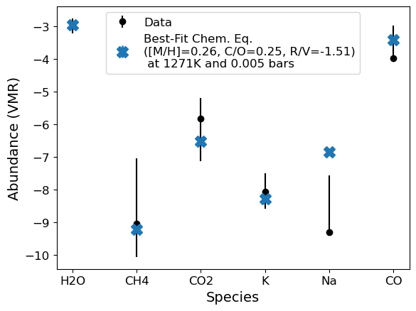
Let’s look at an actual example. Louie et al. 2025
[17]:
#WASP-17b
g = Abund(species_abunds={'H2O':-2.96,'CH4':-9.05,'CO2':-5.81,'K':-8.07,'Na':-9.31,'CO':-3.97},
species_errs={'H2O':[0.24,0.21],'CH4':[1.01,2.01],'CO2':[1.31,0.62],'K':[0.52,0.58],'Na':[0,1.75],'CO':[0,1.0]},
solar='Asplund09')
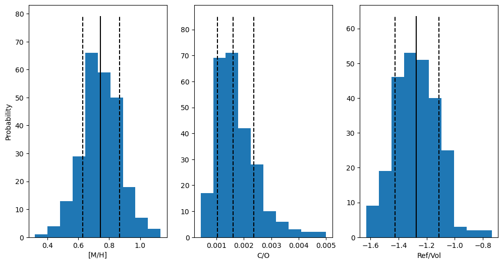
g.convert_species_abunds(1271, 5e-3,plot_it=True,fit_refvol=True)
#g.convert_species_abunds(1271, 5e-3,plot_it=True,fit_refvol=False,adjust_C=False)
#g.convert_species_abunds(1271, 5e-3,plot_it=True,fit_refvol=False,adjust_C='Neither')
plt.savefig('WASP17b_exocomp.pdf')
Optimization terminated successfully.
         Current function value: 2.778314
         Iterations: 96
         Function evaluations: 173
---
Best fit [M/H]: 0.260
Best fit C/O: 0.255
Best fit R/V: -1.509
Chi^2 = 22435859.901501104, Reduced Chi^2 = 4487171.980300221
---
Best Fit Abundances
---
H2O: -2.948740454529697
CH4: -9.205096976006793
CO2: -6.508029084442246
K: -8.287357035986236
Na: -6.846880531894575
CO: -3.411282129239243
Updating bulk abundances with mean/median fit
WASP-178b
WASP-178b is an ultra-hot Jupiter with an observed transit spectrum ranging from 0.2 to 5.1 \(\mu\)m, with detections of refractories and volatiles. Here, we mostly ascribe the large NUV absorption to SiO, but not that it could also be from atomic species like Fe and Mg (and their ions), or some combination of each. In any case, we show here the constraints we would place on the bulk abundances from results from a free retrieval (with posteriors!) and compare them to an equivalent chemical equilibrium retrieval. Remember, as above, the challenge for ultra-hot Jupiters is dealing with thermal dissociation, where some (or lots) of the H\(_2\)O will have dissociated, making it challenging to infer a bulk O/H from measurements of H\(_2\)O.
These retrievals correspond to the isothermal free retrieval case for the combined HST+JWST dataset from Lothringer et al. 2025. These retrievals were run with pRT, so let’s take the posterior, for which the abundances will be in mass fractions, convert them to volume mixing ratios with ExoComp, and fit bulk abundances to them. The standard deviation of the posterior is used as a weight for the fits to each sample- otherwise unconstrained species blow up the constraint on the bulk abundances
(the same problem when trying to infer bulk abundances by adding up atoms per species!).
[2]:
samples_free = np.genfromtxt('W178_eqchem_JWST_retrieval_10bin_1000LP_iso_new_offs_hot_post_equal_weights.dat')

#Columns are: UV offset, IR offset, radius, temperature, log10Pcloud, H2O, CO, CO2, FeH, SiO, TiO, VO, Fe, Fe+, Mg, Mg+
species = ['H2O','CO','CO2','FeH', 'SiO', 'TiO', 'VO', 'Fe', 'Fe+', 'Mg', 'Mg+']
# Unfortunately, these ion species are not included in EasyChem by default
# They can be added manually though with the right thermochemical info
not_included = ['Fe+','Mg+']
offset = 5
posterior_dict_mmw = {}
for i,s in enumerate(species):
    if s in not_included:
        continue
    posterior_dict_mmw[s] = samples_free[:,offset+i]

g = Abund()
posterior_dict_vmr = g.MMR_to_VMR(posterior_dict_mmw, mmw=2.3)

# Make a dict of the median values to input into ExoComp- only used for reference,
# it is the posteriors that matter!
median_dict = {}
for i,s in enumerate(species):
    if s in not_included:
        continue
    median_dict[s] = np.median(posterior_dict_vmr[s])
print('Median VMRs:')
print(median_dict)
Median VMRs:
{'H2O': -6.259975908812065, 'CO': -5.441280282739208, 'CO2': -9.6259416793431, 'FeH': -6.399704413781108, 'SiO': -5.084753936621808, 'TiO': -10.732461397889557, 'VO': -10.288929797996929, 'Fe': -6.447413285227768, 'Mg': -6.000271813664576}
[3]:
g.species_abunds = median_dict
g.species_errs = posterior_dict_vmr
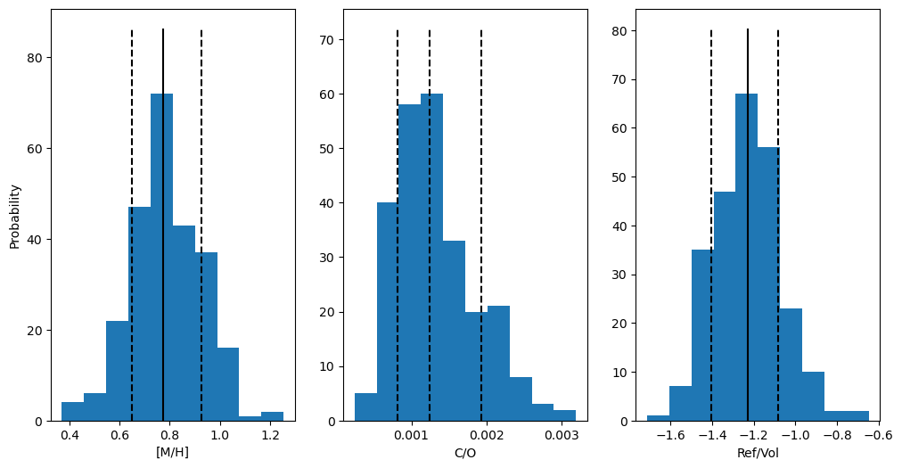
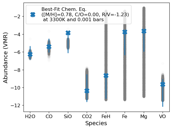
popt,pcov,best_fit = g.convert_species_abunds(3300, 1e-3, plot_it=True,fit_refvol=True, posterior_samples=250)
plt.savefig('WASP178b_exocomp.pdf')
Running on 250 samples... May take a moment if >10
---
Metallicity - Median: 0.7425, Lower bound: 0.6285, Upper bound: 0.8657
C/O - Median: 0.0016, Lower bound: 0.0010, Upper bound: 0.0024
Ref/Vol - Median: -1.2740, Lower bound: -1.4248, Upper bound: -1.1135
---
Median Fit Abundances
---
H2O: -6.342546942879467 + 0.6073334415111322 - 0.8608469086508288
CO: -5.397260058990113 + 0.6274025678119353 - 0.8585983812006326
CO2: -10.434123844104665 + 1.236983028705236 - 1.7336802832130527
FeH: -8.719915084214614 + 2.7423852130688697 - 0.15434695463802584
SiO: -3.9908787457581734 + 2.38025601660468 - 0.14779824058628188
TiO: -7.622897024195767 + 2.4933889945239756 - 0.33218304283236755
VO: -9.906240568173741 + 2.504401867489605 - 0.45163656039393274
Fe: -3.808756048235038 + 2.742623297449149 - 0.15444587903315243
Mg: -3.6916531144848 + 2.3871840172824914 - 0.1507595418080423
Updating bulk abundances with mean/median fit
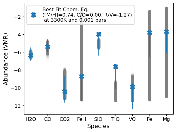
TiO appears to be depleted relative to our chemical equilibrium expectations. This is seen in measurements of other planets too (CITE). It seems likely that some cold-trapping process is depleting Ti-species. Let’s run again, without TiO since we have a prior expectation that our measurement of its abundance in WASP-178b may not be representative of the planet’s bulk composition.
[18]:
#Try without TiO
ss = ['H2O','CO','SiO','CO2','FeH','Fe','Mg','VO']
median_dict_tmp = {}
posterior_dict_vmr_tmp = {}
for s in ss:
    median_dict_tmp[s] = median_dict[s]
    posterior_dict_vmr_tmp[s] = posterior_dict_vmr[s]
g.species_abunds = median_dict_tmp
g.species_errs = posterior_dict_vmr_tmp
popt,pcov,best_fit = g.convert_species_abunds(3300, 1e-3, plot_it=True,fit_refvol=True, posterior_samples=250)
Running on 250 samples... May take a moment if >10
---
Metallicity - Median: 0.7751, Lower bound: 0.6493, Upper bound: 0.9263
C/O - Median: 0.0012, Lower bound: 0.0008, Upper bound: 0.0019
Ref/Vol - Median: -1.2309, Lower bound: -1.4031, Upper bound: -1.0850
---
Median Fit Abundances
---
H2O: -6.257227796699308
CO: -5.408058377209647
SiO: -3.8292797052021577
CO2: -10.349956032933735
FeH: -8.65325791637293
Fe: -3.7372753887939774
Mg: -3.6439448402690777
VO: -9.643689682077227
Updating bulk abundances with mean/median fit
Nice! The best-fit values are pretty consistent with the chemical equilibrium retrievals, which found [O/H] = \(0.4^{+0.45}_{-0.43}\), C/O = \(0.01^{+0.01}_{-0.00}\), and [Si/O] = \(-0.18 \pm 0.49\). The constraints from the chemical equilibrium retrieval are less constraining because they marginalize over the uncertainty in the temperature which is really important (see below)!
A few caveats: 1) The R/V found here adds the contribution of the other refractories, including TiO, which is likely cold-trapped (CITE Pelletier, Gandhi) so it is no surprise that we find a somewhat lower R/V compared to the Si/O measured in the chemical equilibrium retrievals. 2) As described above, these results are sensitive to the temperature and pressure we assume, which is especially true here because of thermal dissociation. If the temperature was a bit higher, we’d infer a higher [O/H] because there’d be more dissociation, while for a lower temperature, we’d infer the opposite. E.g.:
[19]:
print('100 K Hotter')
popt,pcov,best_fit = g.convert_species_abunds(3400, 1e-3, plot_it=False,fit_refvol=True, posterior_samples=250)

print('\n100 K Cooler')
popt,pcov,best_fit = g.convert_species_abunds(3200, 1e-3, plot_it=False,fit_refvol=True, posterior_samples=250)
100 K Hotter
Running on 250 samples... May take a moment if >10
---
Metallicity - Median: 1.2170, Lower bound: 1.0883, Upper bound: 1.3621
C/O - Median: 0.0005, Lower bound: 0.0003, Upper bound: 0.0007
Ref/Vol - Median: -1.6880, Lower bound: -1.8540, Upper bound: -1.5379
---
Median Fit Abundances
---
H2O: -6.273257233938325
CO: -5.407219508416903
SiO: -3.372907870307618
CO2: -10.155719954411932
FeH: -8.303757427011279
Fe: -3.2984350075674014
Mg: -3.206185961570291
VO: -9.064218282698473
Updating bulk abundances with mean/median fit

100 K Cooler
Running on 250 samples... May take a moment if >10
---
Metallicity - Median: 0.2877, Lower bound: 0.1574, Upper bound: 0.4495
C/O - Median: 0.0040, Lower bound: 0.0027, Upper bound: 0.0059
Ref/Vol - Median: -0.7210, Lower bound: -0.8772, Upper bound: -0.5546
---
Median Fit Abundances
---
H2O: -6.267570637248643
CO: -5.391099784632492
SiO: -4.343501020158031
CO2: -10.559576363895035
FeH: -9.047700767974849
Fe: -4.223540242754351
Mg: -4.128453451408211
VO: -10.300507326164016
Updating bulk abundances with mean/median fit
[ ]: